AWS Data Pipeline is a managed web service from Amazon Web Services that automates the movement and transformation of data between different AWS services and on-premises data sources. It lets you define data-driven workflows where tasks run on a schedule and depend on the successful completion of previous tasks — essentially an orchestration layer for ETL (Extract, Transform, Load) jobs across your AWS infrastructure.
However, there is one critical update every developer and data engineer should know: AWS Data Pipeline is now deprecated. The service is in maintenance mode and is no longer available to new customers. In this guide, we cover everything about AWS Data Pipeline — how it works, its components, pricing, real-world use cases — and, most importantly, how to build a modern serverless data pipeline using EMR Serverless, SageMaker Pipelines, Lambda, SQS, and the Medallion Architecture on S3.
AWS Data Pipeline is a cloud-based data workflow orchestration service that was designed to help businesses reliably process and move data at specified intervals. Think of it as a scheduling and execution engine for your data tasks.
At its core, AWS Data Pipeline allows you to:
The service was originally built to solve a common problem: data sits in different places (databases, file systems, data warehouses), and businesses need to move and transform that data regularly without writing custom scripts for every workflow.
As of 2024, AWS Data Pipeline is no longer available to new customers. Amazon has placed the service in maintenance mode, which means:
This is a significant development that affects any organization currently evaluating data orchestration tools on AWS. If you are starting a new project, you should skip AWS Data Pipeline entirely and choose one of the modern alternatives we cover later in this article.
For existing users, AWS has published migration guides to help transition workloads to services like Amazon MWAA (Managed Workflows for Apache Airflow) and AWS Step Functions.
AWS Data Pipeline operates on a simple but powerful execution model:
The execution follows a dependency graph. If Task B depends on Task A completing successfully, AWS Data Pipeline enforces that ordering automatically.
AWS Data Pipeline uses a time-based scheduling model. You define a schedule (for example, “run every day at 2 AM UTC”), and the pipeline creates a new execution instance for each scheduled run. Each instance processes data independently, making it easy to track success or failure for specific time windows.
Understanding the core components is essential to grasping how AWS Data Pipeline works:
The pipeline definition is the blueprint of your data workflow. It is a JSON document that describes all the objects in your pipeline — data sources, destinations, activities, schedules, and their relationships.
Data nodes define where your data lives — both the input source and the output destination:
Activities define the work your pipeline performs:
Task Runners are lightweight agents that poll AWS Data Pipeline for scheduled tasks. When a task is ready, the Task Runner executes it on the assigned compute resource.
Preconditions are checks that must pass before a pipeline activity executes. For example, you might verify a source file exists in S3 before attempting to process it.
Schedules define when your pipeline runs. You configure the start time, frequency, and end time. AWS Data Pipeline supports both one-time and recurring schedules.
Before its deprecation, AWS Data Pipeline was commonly used for these scenarios:
Scenario: An online retailer needs to analyze sales performance across product categories and regions.
Every night at 2 AM, the pipeline extracts order data from their production RDS database, joins it with the product catalog stored in DynamoDB, aggregates sales by category and region, and loads the summary into Amazon Redshift.
Pipeline flow: RDS → EC2 (transform & join) → Redshift
Business value: The marketing team opens their dashboard every morning and sees yesterday’s revenue breakdown by category, top-selling products, and regional performance — all without a single manual SQL query.
Scenario: A SaaS company with 50 EC2 instances running Nginx wants to understand their traffic patterns.
The pipeline collects access logs from all instances daily, archives them to S3, and runs a weekly EMR job that processes the logs to generate reports: top pages by traffic, error rate trends, geographic distribution, and peak usage hours.
Pipeline flow: EC2 logs → S3 (daily archive) → EMR (weekly analysis) → S3 (reports)
Business value: The engineering team spots a 3x increase in 404 errors from mobile users, leading them to discover and fix a broken API endpoint that was costing them 12% of mobile traffic.
Scenario: A hospital network runs their patient management system on an on-premises SQL Server database but wants their analytics team to work in AWS.
Every 6 hours, the pipeline syncs patient appointment data from the on-premises database to AWS RDS using the Task Runner installed on a local server. The data then feeds into Redshift for operational analytics.
Pipeline flow: On-premises SQL Server → Task Runner → RDS → Redshift
Business value: Compliance-friendly data movement with full audit trails. The analytics team can predict patient no-show rates and optimize scheduling without touching the production database.
Scenario: A fintech company must generate regulatory reports every quarter, which requires combining transaction data with compliance rules.
The pipeline extracts transaction records from DynamoDB, runs them through an EMR cluster that applies PII masking (replacing real names with hashes), converts currencies to USD, validates against compliance rules, and loads the clean dataset into Redshift.
Pipeline flow: DynamoDB → EMR (PII masking + currency conversion) → Redshift
Business value: What used to take a compliance team 2 weeks of manual work now runs automatically in 4 hours, with consistent results every quarter.
Scenario: A global company with teams in the US and EU needs both teams to have access to fresh analytics data, but running cross-region queries is too slow and expensive.
The pipeline replicates the daily S3 data from us-east-1 to eu-west-1 on a nightly schedule, so the European team queries local data with low latency.
Pipeline flow: S3 (us-east-1) → S3 (eu-west-1)
Business value: EU analysts get sub-second query times instead of 30-second cross-region queries, and data transfer costs are predictable since it runs on a fixed schedule rather than on-demand.
AWS Data Pipeline pricing is based on how frequently your activities run:
| Activity Type | Cost |
|---|---|
| Low-frequency activity (runs once per day or less) | $0.60 per activity per month |
| High-frequency activity (runs more than once per day) | $1.00 per activity per month |
| Low-frequency precondition | $0.60 per precondition per month |
| High-frequency precondition | $1.00 per precondition per month |
New AWS accounts (less than 12 months old) qualify for the AWS Free Tier:
Important: AWS Data Pipeline pricing covers only the orchestration. You still pay separately for the underlying compute (EC2 instances, EMR clusters) and storage (S3, RDS, Redshift) that your pipeline uses.
| Pros | Cons |
|---|---|
| Native AWS integration with S3, RDS, DynamoDB, Redshift, EMR | Deprecated — no new features or region support |
| Built-in retry and fault tolerance | Dated UI and developer experience |
| Supports on-premises data sources via Task Runner | Limited to batch processing — no real-time support |
| Schedule-based automation with dependency management | Debugging failed jobs is difficult |
| Low orchestration cost | Lock-in to AWS ecosystem |
| Visual pipeline designer in console | JSON-based definitions are verbose and hard to maintain |
Since AWS Data Pipeline is deprecated, here are the recommended alternatives:
Amazon MWAA is the most direct replacement. It is a fully managed Apache Airflow service that handles the infrastructure for running Airflow workflows.
Best for: Complex, multi-step ETL workflows with branching logic and dynamic task generation.
AWS Step Functions is a serverless orchestration service that coordinates AWS services using visual workflows.
Best for: Serverless architectures, event-driven processing, and workflows that integrate with Lambda functions.
Amazon EventBridge is an event bus that triggers workflows based on events from AWS services, SaaS applications, or custom sources.
Best for: Event-driven architectures where data processing starts in response to specific triggers.
| Feature | AWS Data Pipeline | AWS Step Functions |
|---|---|---|
| Status | Deprecated (maintenance mode) | Actively developed |
| Execution model | Schedule-based | Event-driven or schedule-based |
| Compute | EC2, EMR | Lambda, ECS, any AWS service |
| Serverless | No (requires EC2/EMR) | Yes (fully serverless) |
| Pricing | Per activity per month | Per state transition |
| Visual editor | Basic | Advanced (Workflow Studio) |
| Error handling | Retry with notifications | Catch, retry, fallback states |
| Real-time support | No | Yes |
For most new projects, AWS Step Functions is the better choice due to its serverless nature and active development.
No, AWS Data Pipeline is not serverless. It requires provisioning EC2 instances or EMR clusters to execute pipeline activities. The Task Runner agent must run on compute resources that you manage.
This is a key difference from modern alternatives like AWS Step Functions, which are fully serverless — you define your workflow, and AWS handles everything else.
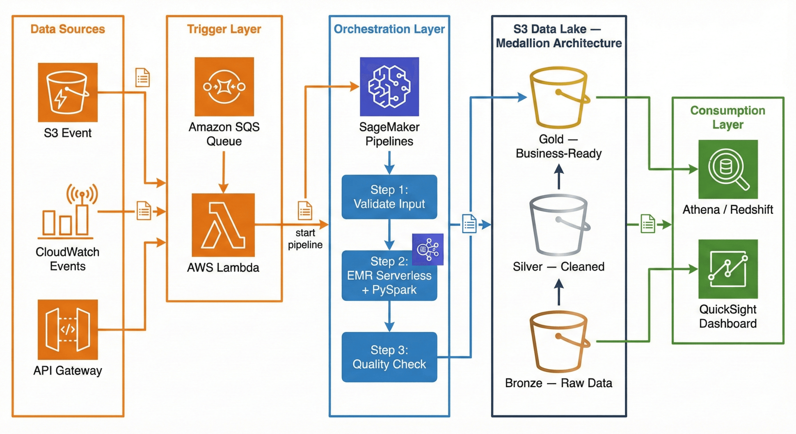
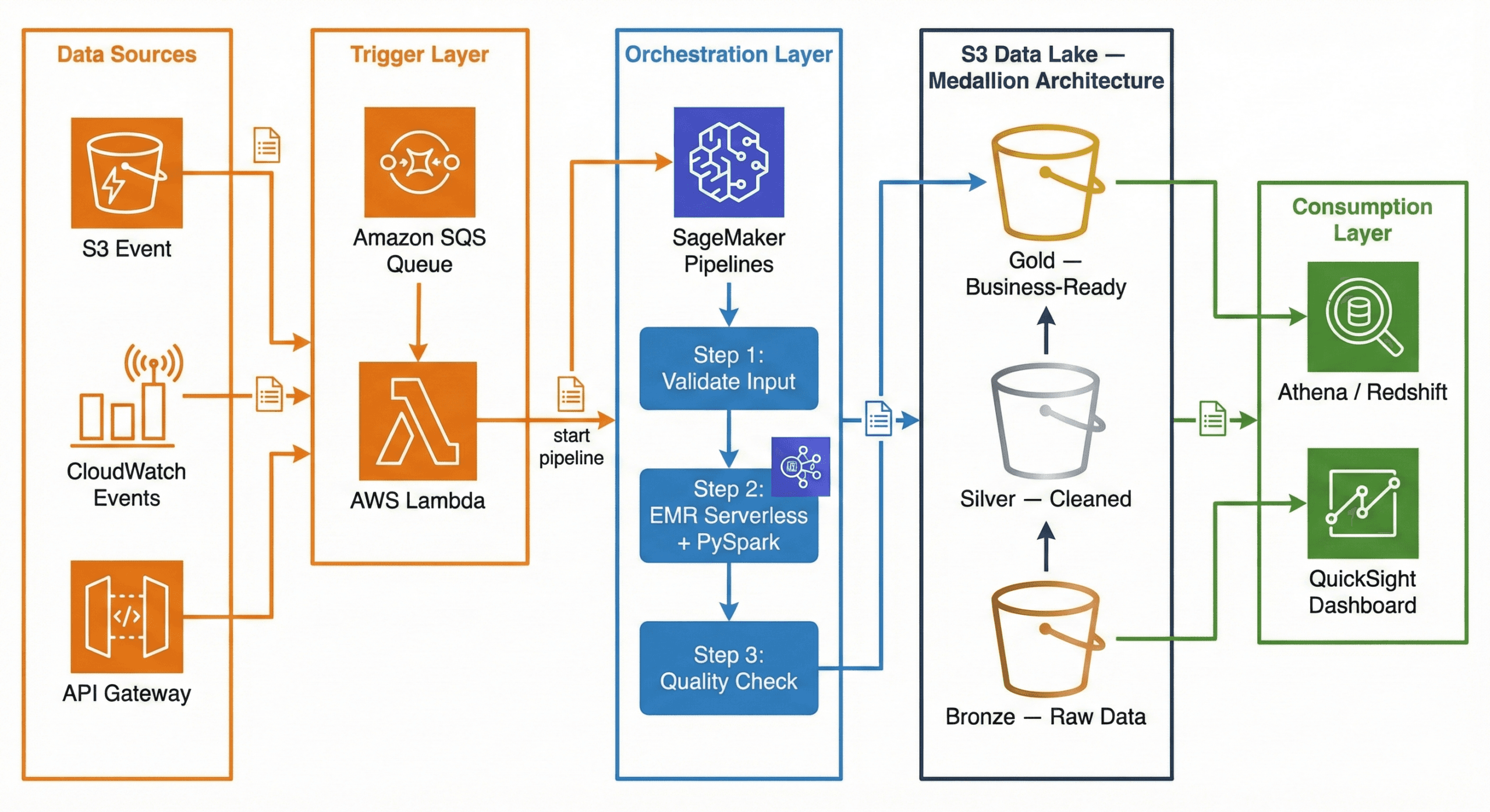
Now that AWS Data Pipeline is deprecated, what does a modern data pipeline look like on AWS? Here is a production-ready architecture using current AWS services:
┌─────────────┐     ┌─────────────┐     ┌──────────────────────┐
│ Data Sources │     │  CloudWatch  │     │   API Gateway /      │
│  (S3 Event)  │────▶│  Events      │────▶│   External Triggers  │
└──────┬───────┘     └──────┬───────┘     └──────────┬───────────┘
       │                    │                        │
       ▼                    ▼                        ▼
┌──────────────────────────────────────────────────────────────┐
│                     Amazon SQS (Queue)                       │
│              Decouples triggers from processing              │
└──────────────────────────┬───────────────────────────────────┘
                           │
                           ▼
┌──────────────────────────────────────────────────────────────┐
│                    AWS Lambda (Trigger)                       │
│         Validates event, starts SageMaker Pipeline           │
└──────────────────────────┬───────────────────────────────────┘
                           │
                           ▼
┌──────────────────────────────────────────────────────────────┐
│              Amazon SageMaker Pipelines                      │
│                   (Orchestration)                             │
│                                                              │
│  ┌──────────┐   ┌───────────────┐   ┌────────────────────┐  │
│  │  Step 1:  │──▶│    Step 2:     │──▶│      Step 3:       │  │
│  │ Validate  │   │ EMR Serverless │   │  Quality Check     │  │
│  │  Input    │   │  + PySpark     │   │  + Write to Gold   │  │
│  └──────────┘   └───────────────┘   └────────────────────┘  │
└──────────────────────────────────────────────────────────────┘
                           │
                           ▼
┌──────────────────────────────────────────────────────────────┐
│                    Amazon S3 Data Lake                        │
│                                                              │
│  ┌────────────┐   ┌────────────┐   ┌─────────────────────┐  │
│  │   Bronze    │──▶│   Silver    │──▶│       Gold          │  │
│  │ (Raw Data)  │   │ (Cleaned)   │   │ (Business-Ready)   │  │
│  └────────────┘   └────────────┘   └─────────────────────┘  │
└──────────────────────────────────────────────────────────────┘
                           │
                    ┌──────┴──────┐
                    ▼             ▼
             ┌───────────┐  ┌──────────┐
             │ Redshift / │  │ QuickSight│
             │  Athena    │  │ Dashboard │
             └───────────┘  └──────────┘
Trigger Layer — Lambda + SQS:
When a new file lands in S3 (or a scheduled CloudWatch Event fires), the event goes to an SQS queue. A Lambda function picks it up, validates the event, and kicks off the SageMaker Pipeline. Why SQS in between? It decouples the trigger from the processing. If the pipeline is busy, messages wait in the queue instead of being lost. If something fails, the message goes to a dead-letter queue for investigation.
Orchestration Layer — SageMaker Pipelines:
SageMaker Pipelines manages the end-to-end workflow. It defines each step as a node in a directed acyclic graph (DAG), handles retries, caches intermediate results, and provides a visual interface to monitor progress. While SageMaker is known for machine learning, its pipeline orchestration works perfectly for general-purpose data engineering too.
Processing Layer — EMR Serverless + PySpark:
Amazon EMR Serverless runs your PySpark jobs without you ever touching a cluster. You submit your Spark code, EMR Serverless provisions the exact resources needed, runs the job, and shuts down. You pay only for the compute time used. No cluster management, no idle costs, and it auto-scales based on your data volume.
Storage Layer — S3 Data Lake (Medallion Architecture):
Data flows through three layers in S3: Bronze (raw), Silver (cleaned), Gold (business-ready). This is called the Medallion Architecture, and we explain it in full detail in the next section.
Consumption Layer — Athena / Redshift + QuickSight:
Once data reaches the Gold layer, analysts query it using Amazon Athena (serverless SQL directly on S3) or Amazon Redshift (data warehouse). QuickSight dashboards visualize the results for business stakeholders.
The Medallion Architecture is the most popular pattern for organizing data in a data lake. If you have ever struggled with messy, unreliable data, this pattern will make your life significantly easier.
Think of it like a kitchen:
In data terms:
| Layer | What It Contains | Who Uses It |
|---|---|---|
| Bronze | Raw data exactly as received from the source | Data engineers (debugging, reprocessing) |
| Silver | Cleaned, validated, deduplicated data with enforced schema | Data analysts, data scientists |
| Gold | Aggregated, business-ready tables optimized for dashboards | Business users, executives, BI tools |
Why not just clean the data once and store it? Because requirements change. A business rule that seems right today might be wrong next month. By keeping the raw data in Bronze, you can always go back and reprocess it with new logic. You never lose the original truth.
Here is the actual folder structure you would create in your S3 bucket. This is what a production data lake looks like:
s3://mycompany-data-lake/
│
├── bronze/
│   ├── orders/
│   │   ├── dt=2026-02-10/
│   │   │   └── orders_raw_001.json
│   │   ├── dt=2026-02-11/
│   │   │   └── orders_raw_001.json
│   │   └── dt=2026-02-12/
│   │       └── orders_raw_001.json
│   ├── customers/
│   │   └── dt=2026-02-12/
│   │       └── customers_export.csv
│   └── products/
│       └── dt=2026-02-12/
│           └── products_catalog.json
│
├── silver/
│   ├── orders/
│   │   └── dt=2026-02-12/
│   │       └── part-00000.snappy.parquet
│   ├── order_items/
│   │   └── dt=2026-02-12/
│   │       └── part-00000.snappy.parquet
│   ├── customers/
│   │   └── dt=2026-02-12/
│   │       └── part-00000.snappy.parquet
│   └── products/
│       └── dt=2026-02-12/
│           └── part-00000.snappy.parquet
│
└── gold/
    ├── fact_daily_sales/
    │   └── dt=2026-02-12/
    │       └── part-00000.snappy.parquet
    ├── dim_customer/
    │   └── part-00000.snappy.parquet
    ├── dim_product/
    │   └── part-00000.snappy.parquet
    └── dim_date/
        └── part-00000.snappy.parquet
Why this structure?
dt=YYYY-MM-DD partitioning — Each date gets its own folder. This makes it trivial to reprocess a specific day or query a date rangeorders/, customers/, products/ are isolated. Each can have its own IAM access policyThe Bronze layer is the simplest. Your only job is to land the data exactly as received and tag it with when it arrived. No cleaning, no transforming, no filtering.
What happens at this stage:
E-commerce example: Your Shopify store sends a webhook with order data as JSON. You receive it and store it immediately.
# ============================================
# BRONZE LAYER: Ingest raw data — no changes
# ============================================
from pyspark.sql import SparkSession
from pyspark.sql.functions import current_timestamp, lit
from datetime import date

spark = SparkSession.builder \
    .appName("bronze-ingestion") \
    .getOrCreate()

today = date.today().isoformat()  # "2026-02-12"

# Read raw JSON from the source — could be an API export, S3 drop, etc.
raw_orders = spark.read.json("s3://source-bucket/shopify-exports/orders.json")

# Add metadata columns (when did we ingest this? from where?)
bronze_orders = raw_orders \
    .withColumn("_ingested_at", current_timestamp()) \
    .withColumn("_source_system", lit("shopify")) \
    .withColumn("_file_name", lit("orders.json"))

# Write to Bronze — append mode, never overwrite historical data
bronze_orders.write \
    .mode("append") \
    .json(f"s3://mycompany-data-lake/bronze/orders/dt={today}/")

print(f"Bronze: {bronze_orders.count()} raw orders ingested for {today}")
Key rules for Bronze:
_ingested_at, _source_system, _file_name help with debuggingThe Silver layer is where the real work begins. You take the messy Bronze data and turn it into something reliable and consistent.
What happens at this stage:
E-commerce example: The raw Shopify JSON has duplicate orders (webhooks sometimes fire twice), some orders have no customer_id, prices are stored as strings, and email addresses have trailing spaces.
# ================================================
# SILVER LAYER: Clean, validate, and standardize
# ================================================
from pyspark.sql.functions import col, to_date, trim, when, explode
from pyspark.sql.types import DecimalType

# Read all Bronze data
bronze_orders = spark.read.json("s3://mycompany-data-lake/bronze/orders/")

print(f"Bronze records: {bronze_orders.count()}")

# ---- STEP 1: Remove duplicates ----
# Shopify webhooks sometimes fire twice for the same order
deduped = bronze_orders.dropDuplicates(["order_id"])

# ---- STEP 2: Drop invalid records ----
# Orders without order_id or customer_id are useless
valid = deduped.filter(
    col("order_id").isNotNull() &
    col("customer_id").isNotNull()
)

# ---- STEP 3: Enforce data types ----
typed = valid \
    .withColumn("total_price", col("total_price").cast(DecimalType(10, 2))) \
    .withColumn("order_date", to_date(col("created_at")))

# ---- STEP 4: Clean string fields ----
cleaned = typed \
    .withColumn("email", trim(col("email"))) \
    .withColumn("shipping_country",
        when(col("shipping_country").isNull(), "Unknown")
        .otherwise(trim(col("shipping_country")))
    )

# ---- STEP 5: Write to Silver as Parquet ----
cleaned.write \
    .mode("overwrite") \
    .partitionBy("order_date") \
    .parquet("s3://mycompany-data-lake/silver/orders/")

removed = bronze_orders.count() - cleaned.count()
print(f"Silver: {cleaned.count()} clean orders ({removed} bad records removed)")
Flattening nested data (bonus):
Shopify orders contain a line_items array — each order has multiple products. In Bronze, this is stored as a nested array. In Silver, we explode it into separate rows:
# Flatten line_items array into separate rows
order_items = cleaned \
    .select("order_id", "order_date", explode("line_items").alias("item")) \
    .select(
        "order_id",
        "order_date",
        col("item.product_id").alias("product_id"),
        col("item.name").alias("product_name"),
        col("item.quantity").cast("int").alias("quantity"),
        col("item.price").cast(DecimalType(10, 2)).alias("unit_price")
    )

order_items.write \
    .mode("overwrite") \
    .partitionBy("order_date") \
    .parquet("s3://mycompany-data-lake/silver/order_items/")
Why Parquet? A 1GB JSON file becomes ~200MB in Parquet. Queries that used to take 30 seconds now take 3 seconds. Parquet stores data in columns, so when you query only order_date and total_price, it does not read the other 20 columns at all.
The Gold layer is where data becomes useful for business decisions. You join tables, calculate KPIs, and build the datasets that power dashboards.
What happens at this stage:
E-commerce example: Build a daily sales summary that the marketing team can view in QuickSight.
# ================================================
# GOLD LAYER: Aggregate and build business tables
# ================================================
from pyspark.sql.functions import sum, count, avg, round, countDistinct

# Read cleaned data from Silver
orders = spark.read.parquet("s3://mycompany-data-lake/silver/orders/")
order_items = spark.read.parquet("s3://mycompany-data-lake/silver/order_items/")
products = spark.read.parquet("s3://mycompany-data-lake/silver/products/")

# Join order items with product details
enriched = order_items.join(products, "product_id", "left")

# Build daily sales summary
daily_sales = (
    enriched
    .groupBy("order_date", "category")
    .agg(
        round(sum(col("unit_price") * col("quantity")), 2).alias("total_revenue"),
        count("order_id").alias("total_items_sold"),
        countDistinct("order_id").alias("unique_orders"),
        round(avg(col("unit_price") * col("quantity")), 2).alias("avg_item_value")
    )
    .orderBy("order_date", "category")
)

# Write to Gold layer
daily_sales.write \
    .mode("overwrite") \
    .partitionBy("order_date") \
    .parquet("s3://mycompany-data-lake/gold/fact_daily_sales/")

daily_sales.show(5, truncate=False)
Sample output:
+----------+-------------+-------------+----------------+-------------+--------------+
|order_date|category     |total_revenue|total_items_sold|unique_orders|avg_item_value|
+----------+-------------+-------------+----------------+-------------+--------------+
|2026-02-12|Electronics  |45230.50     |312             |156          |145.00        |
|2026-02-12|Clothing     |12450.75     |178             |89           |69.95         |
|2026-02-12|Home & Garden|8920.00      |90              |45           |99.11         |
|2026-02-12|Books        |3240.00      |216             |108          |15.00         |
|2026-02-12|Sports       |6780.25      |67              |34           |101.20        |
+----------+-------------+-------------+----------------+-------------+--------------+
Now your marketing team can open QuickSight, filter by date and category, and see exactly how each product line performed — no SQL knowledge required.
Each layer uses a different modeling approach. Here is why:
| Layer | Modeling Style | What It Looks Like | Why |
|---|---|---|---|
| Bronze | No model (source-as-is) | Raw JSON from Shopify, CSV from CRM | Preserve the original structure for auditing and reprocessing |
| Silver | Normalized (3NF-like) | Separate orders, order_items, customers, products tables with foreign keys |
Remove redundancy, enforce data types, create an enterprise-wide clean dataset |
| Gold | Denormalized (Star Schema) | Central fact_daily_sales table + dim_customer, dim_product, dim_date |
Fast queries, fewer joins, dashboard-ready |
There is no modeling in Bronze. You store exactly what the source sends:
_ingested_at, _source_system, _file_nameIn Silver, you create clean, separate tables with proper relationships:
silver_orders          silver_order_items       silver_customers       silver_products
─────────────          ──────────────────       ────────────────       ───────────────
order_id (PK)          order_item_id (PK)       customer_id (PK)       product_id (PK)
customer_id (FK) ───┐  order_id (FK) ──────┐    name                   name
order_date           │  product_id (FK) ─┐  │    email                  category
total_price          │  quantity         │  │    country                brand
email                │  unit_price       │  │    segment                price
shipping_country     │                   │  │    created_at             sku
status               │                   │  │
                     │                   │  │
                     └───────────────────┘  └── Relationships enforce
                                                data integrity
Key principle: Each piece of information is stored in exactly one place. A customer’s name exists only in silver_customers, not duplicated across every order row.
The Gold layer uses a star schema — one central fact table surrounded by dimension tables, forming a star shape:
                    ┌──────────────┐
                    │  dim_date    │
                    │──────────────│
                    │ date         │
                    │ day_of_week  │
                    │ month        │
                    │ quarter      │
                    │ year         │
                    │ is_weekend   │
                    │ is_holiday   │
                    └──────┬───────┘
                           │
┌──────────────┐   ┌──────┴───────────┐   ┌──────────────┐
│ dim_customer │   │ fact_daily_sales │   │ dim_product  │
│──────────────│   │──────────────────│   │──────────────│
│ customer_id  │◄──│ order_date (FK)  │──▶│ product_id   │
│ name         │   │ customer_id (FK) │   │ name         │
│ segment      │   │ product_id (FK)  │   │ category     │
│ country      │   │ total_revenue    │   │ brand        │
│ lifetime_val │   │ total_orders     │   │ price_tier   │
└──────────────┘   │ avg_order_value  │   └──────────────┘
                   │ quantity_sold    │
                   └──────────────────┘
Why star schema for Gold?
When a business user asks “Show me total revenue by country for Q1 2026,” the query only needs to join fact_daily_sales with dim_customer and dim_date. That is 2 simple joins instead of scanning 5 normalized tables. BI tools like QuickSight, Power BI, and Tableau are specifically optimized for star schemas — they understand facts and dimensions natively.
Partitioning is how you organize files within each layer so that queries only read the data they need instead of scanning everything.
Many tutorials teach the Hive-style year/month/day partitioning:
s3://data-lake/bronze/orders/year=2026/month=02/day=12/
Why this is a problem:
WHERE year=2026 AND month=02 AND day>=10 AND day<=28Use a single date partition key in ISO 8601 format:
s3://data-lake/bronze/orders/dt=2026-02-12/
Why this works better:
WHERE dt BETWEEN '2026-02-01' AND '2026-02-28'| Layer | Partition Key | Example Path | Why |
|---|---|---|---|
| Bronze | dt (ingestion date) |
bronze/orders/dt=2026-02-12/ |
Track when data arrived from the source |
| Silver | dt (business event date) |
silver/orders/dt=2026-02-12/ |
Query by when the business event happened |
| Gold | Business key + date | gold/sales/region=US/dt=2026-02-12/ |
Optimized for common dashboard filter patterns |
dt=2026-W07/| Layer | Format | Compression | Size vs JSON | Why |
|---|---|---|---|---|
| Bronze | JSON or CSV (as received) | None or GZIP | 1x (original) | Preserve the exact source format |
| Silver | Apache Parquet | Snappy | ~0.2x (80% smaller) | Columnar format, fast reads, great compression |
| Gold | Apache Parquet | Snappy | ~0.2x (80% smaller) | Same benefits + optimized for Athena and Redshift Spectrum |
| # | Best Practice | Why It Matters |
|---|---|---|
| 1 | Never delete Bronze data | You can always reprocess with new business rules |
| 2 | Use Parquet + Snappy in Silver/Gold | 70-80% storage savings, 10x faster queries |
| 3 | Single-key date partitioning (dt=YYYY-MM-DD) |
Simpler queries, better partition pruning |
| 4 | S3 Lifecycle policies — Bronze to Infrequent Access after 30 days, Glacier after 90 | Cut storage costs by 50-70% for old data |
| 5 | Register tables in AWS Glue Data Catalog | Athena, Redshift Spectrum, and EMR can all query by table name |
| 6 | Star schema in Gold | BI tools are optimized for fact + dimension tables |
| 7 | Start with one data source | Get orders working end-to-end before adding customers, products, etc. |
| 8 | Add metadata in Bronze (_ingested_at, _source) |
Essential for debugging and data lineage |
If you are currently using AWS Data Pipeline and need to migrate:
ETL (Extract, Transform, Load) is a process — it describes the pattern of pulling data from sources, transforming it, and loading it into a destination. AWS Data Pipeline is a tool that orchestrates ETL processes. The actual extraction, transformation, and loading are performed by other services like EMR, EC2, or Redshift.
For existing customers, yes — it continues to function. However, it is not available to new customers. AWS recommends Amazon MWAA or AWS Step Functions for new projects.
There is no single direct replacement:
Yes, if you are an existing customer. However, you should start planning a migration since the service will not receive new features, and AWS could eventually announce an end-of-life date.
Medallion Architecture organizes data into three layers — Bronze (raw), Silver (cleaned), and Gold (business-ready). Each layer progressively improves data quality. It is the standard pattern for building data lakes on S3.
For most data pipeline use cases, yes. EMR Serverless eliminates cluster management — you submit your PySpark job and AWS handles provisioning, scaling, and termination. You pay only for the compute time used. Use regular EMR only if you need persistent clusters or custom configurations.
AWS Data Pipeline was a pioneering service that introduced many organizations to managed data orchestration on AWS. Its ability to schedule, execute, and monitor data workflows made it a valuable tool for batch processing and ETL automation.
However, with the service now in maintenance mode and unavailable to new customers, it is time to build with modern tools. The combination of SageMaker Pipelines for orchestration, EMR Serverless with PySpark for processing, Lambda + SQS for triggering, and the Medallion Architecture on S3 for storage gives you a production-ready, serverless, and cost-efficient data pipeline that scales from gigabytes to petabytes.
Whether you are building your first data pipeline or migrating from a legacy system, the key principles remain the same: keep your raw data safe in Bronze, clean it thoroughly in Silver, and serve it beautifully in Gold.
Need help building modern data pipelines on AWS? At Metosys, we specialize in ETL pipeline development, AWS data engineering with Glue and Redshift, and workflow automation with Apache Airflow. Our data engineers can help you migrate from legacy systems or build new pipelines from scratch. Get in touch to discuss your project.
Sources:
Was this article helpful?

Stay in the know with insights from industry experts.